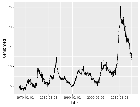

<ggplot: (383084815)>English
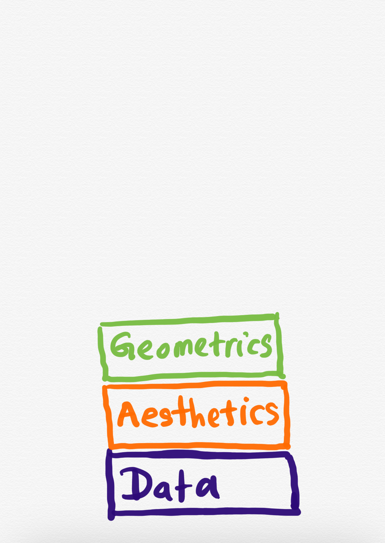
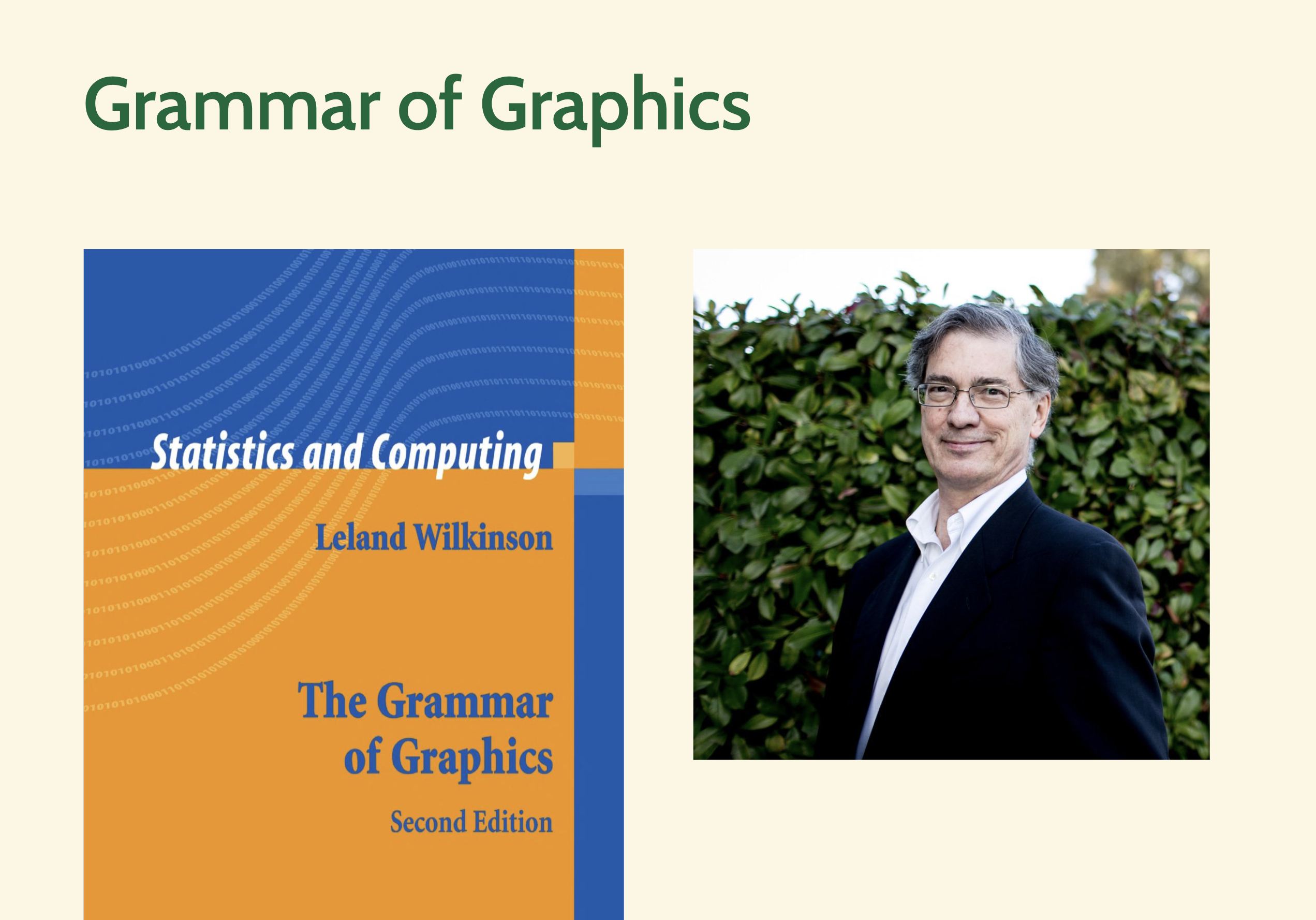
Graphics
English
The little monkey hangs confidently by a branch.
Graphics
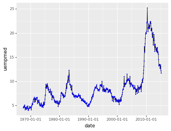
<ggplot: (383084815)>English
Article: The
Adjective: little
Noun: monkey
Verb: hangs
Adverb: Confidently
Proposition: by
Noun: a branch
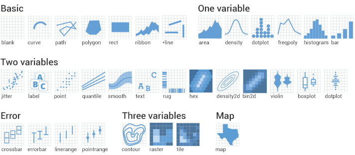
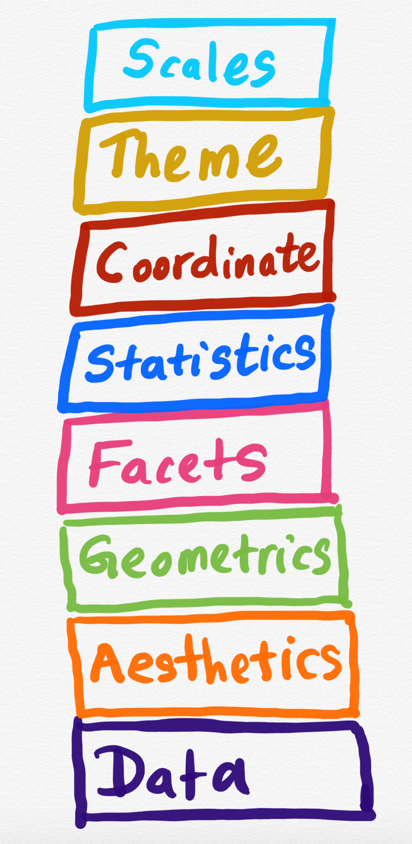
Graphics
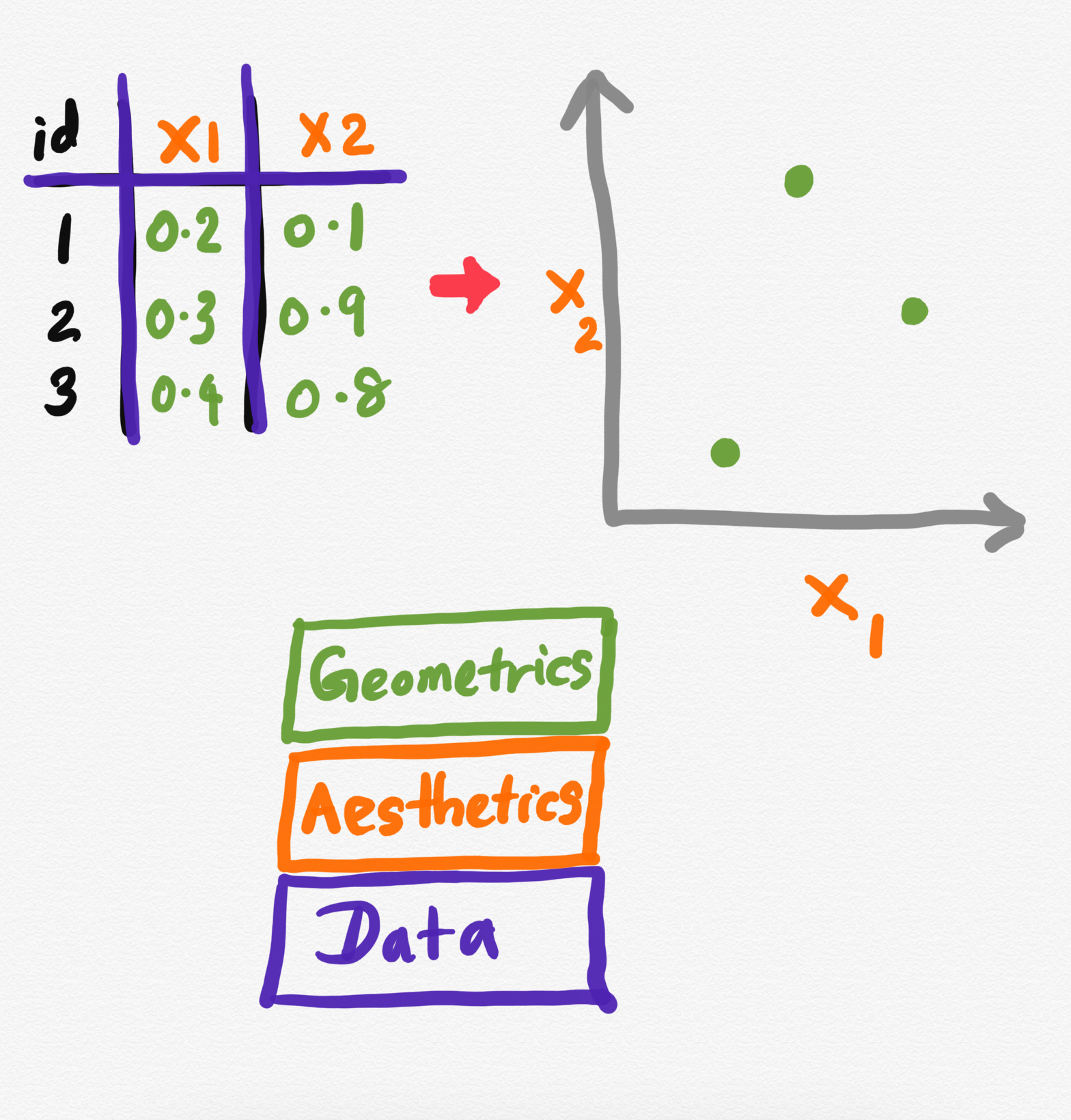
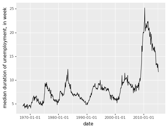
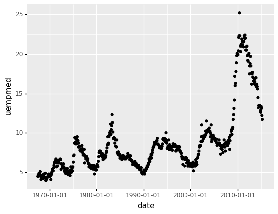
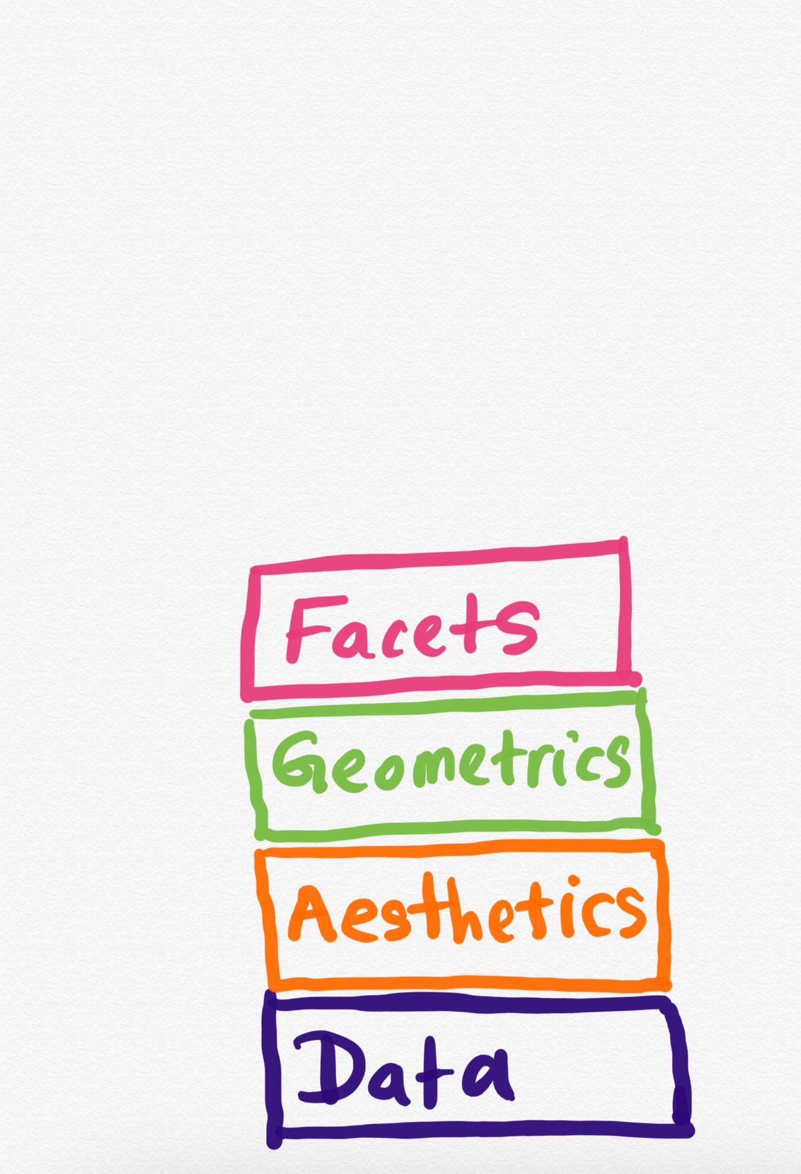
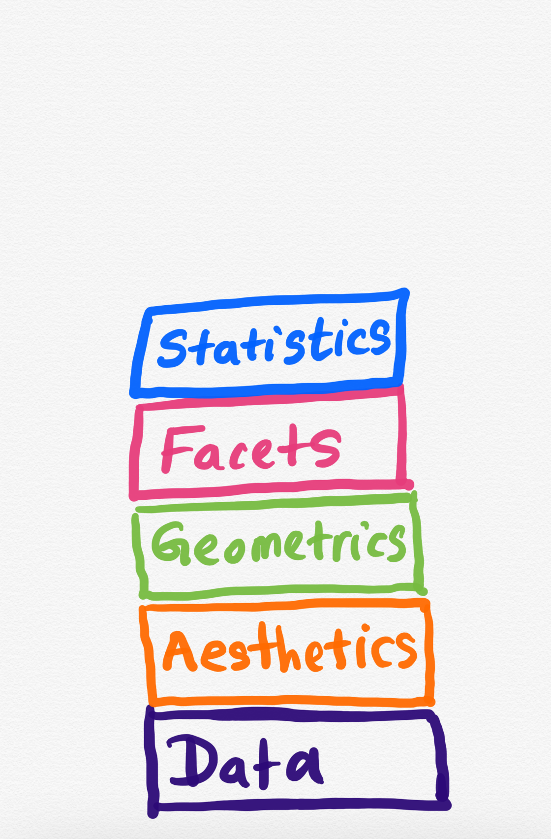
geom_linegeom_pointDate: data to be plotted
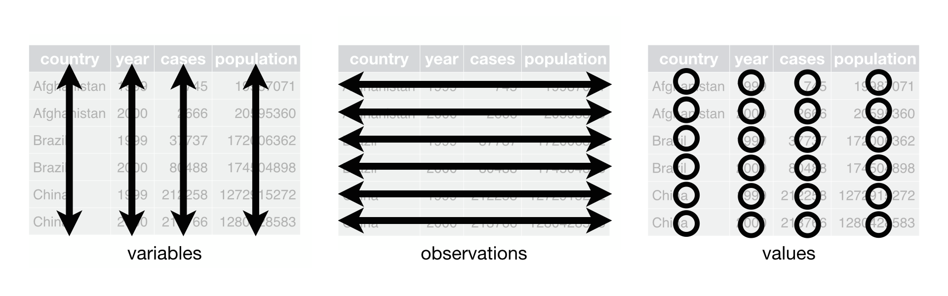
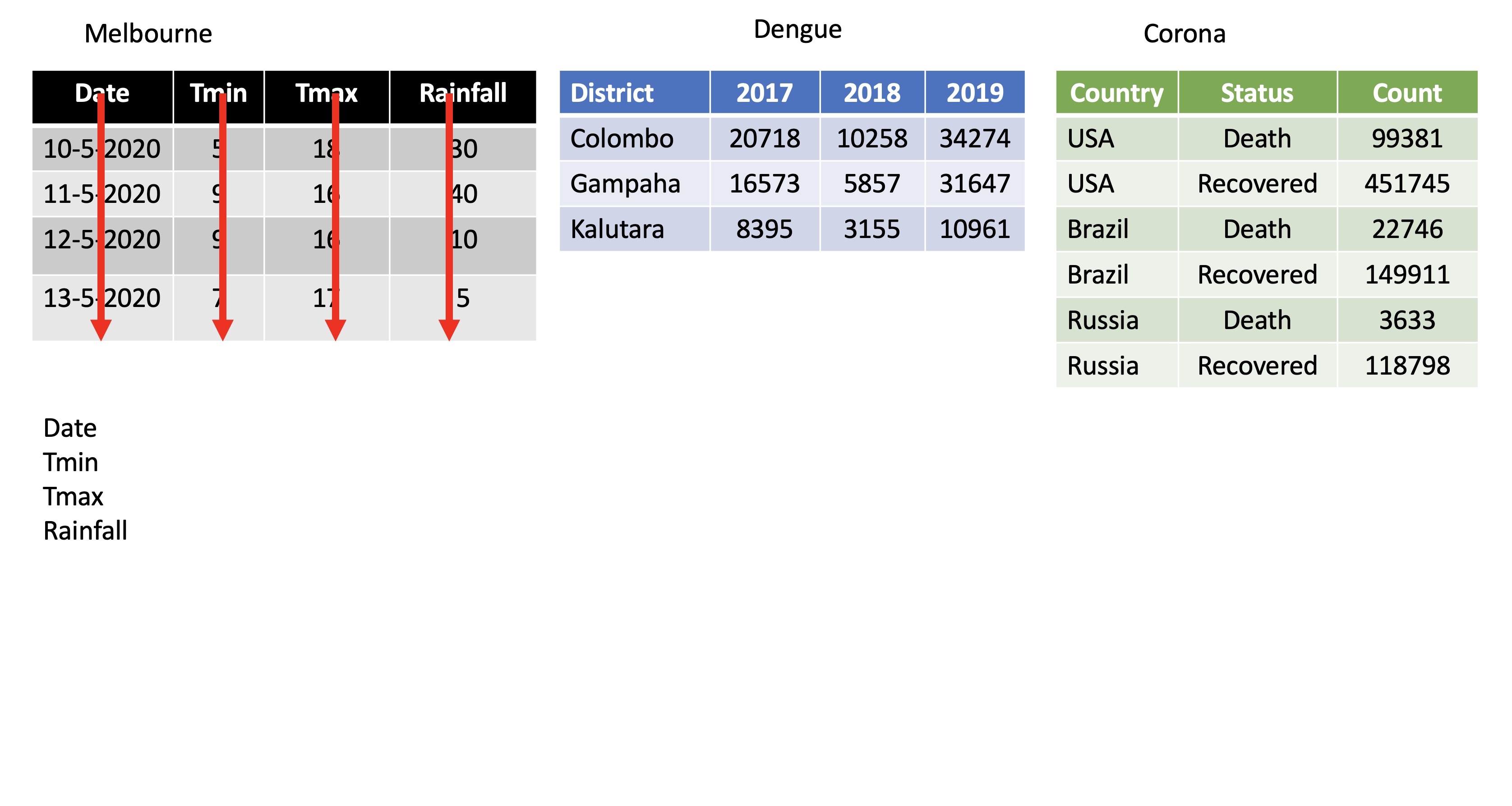
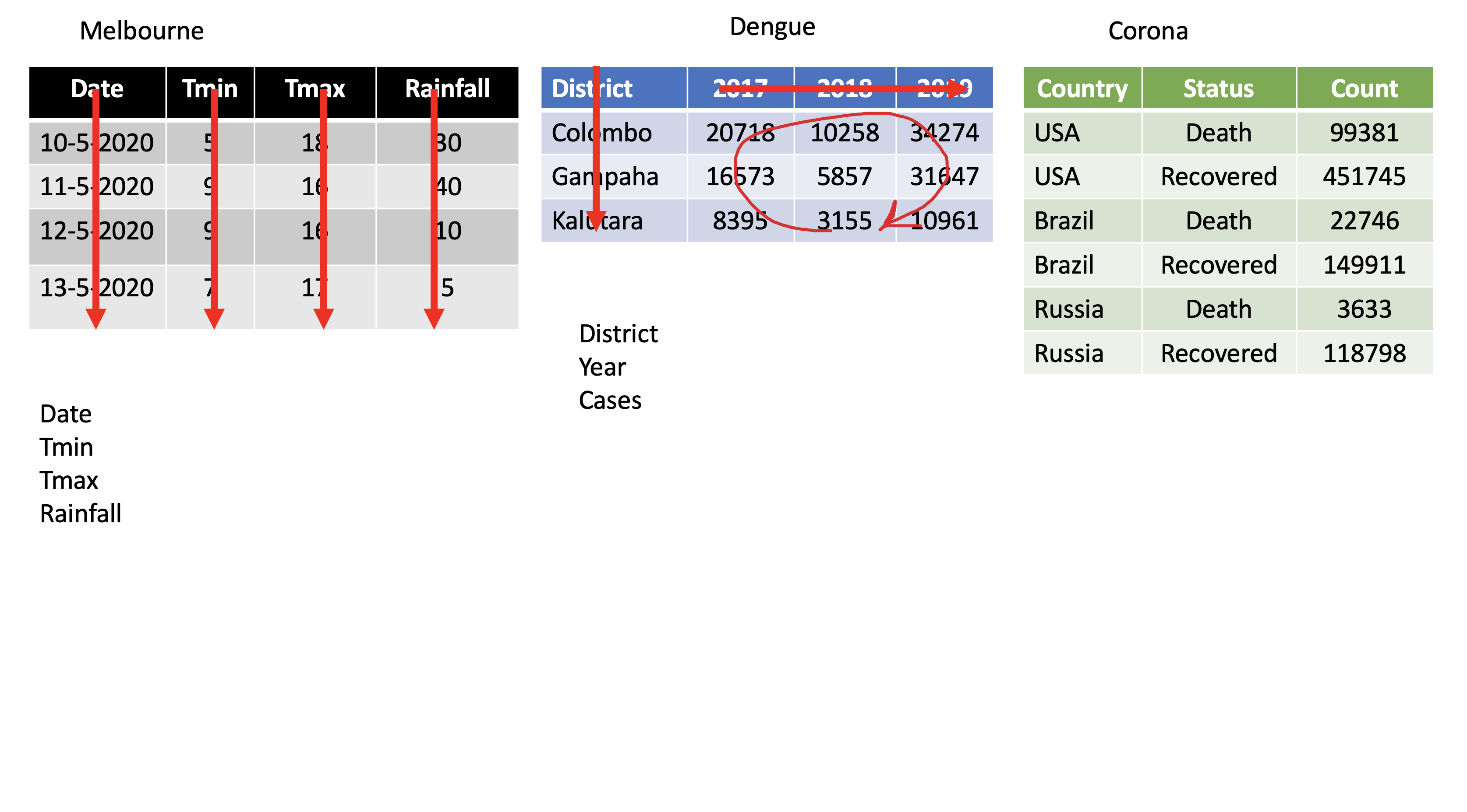
Every column is a variable.
Every row is an observation.
Every cell is a single value.
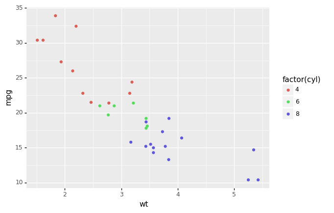
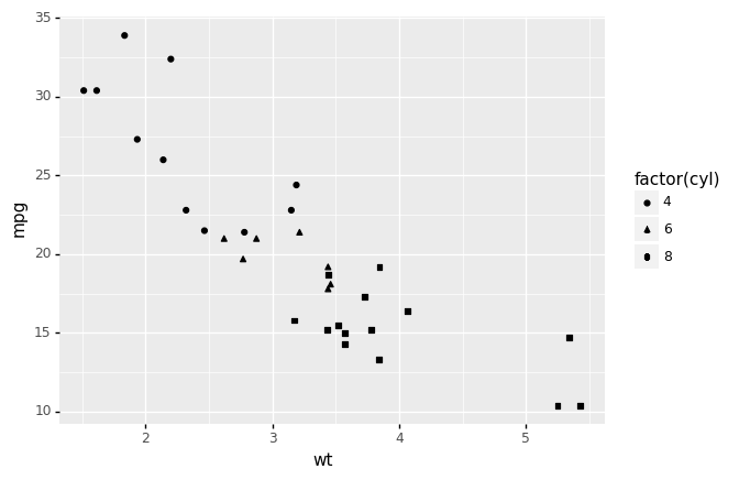
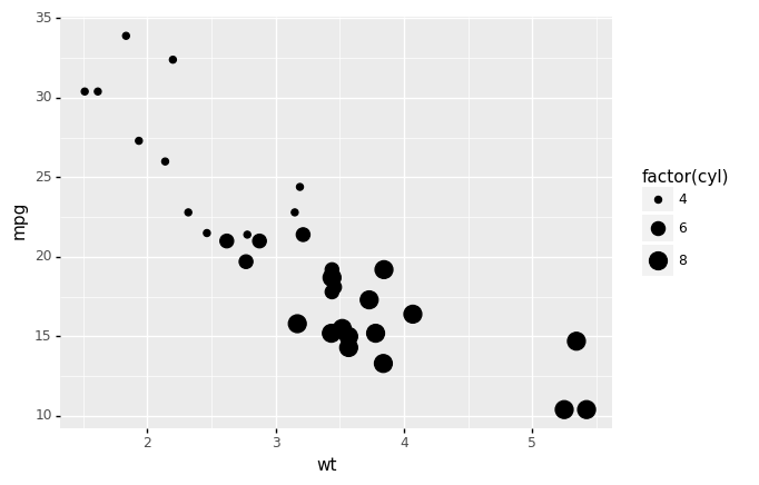
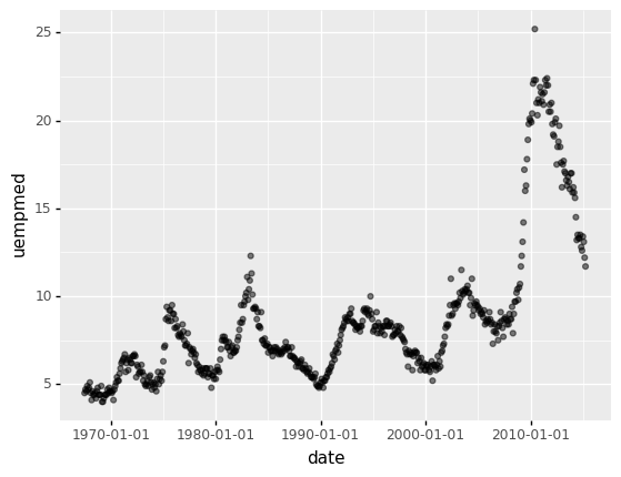
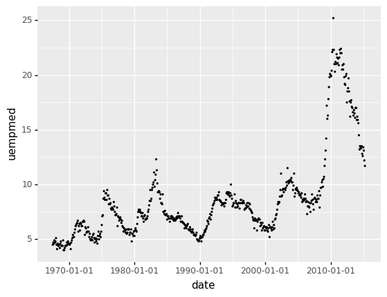
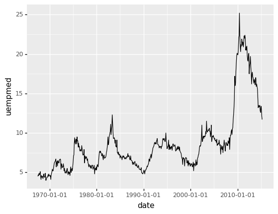
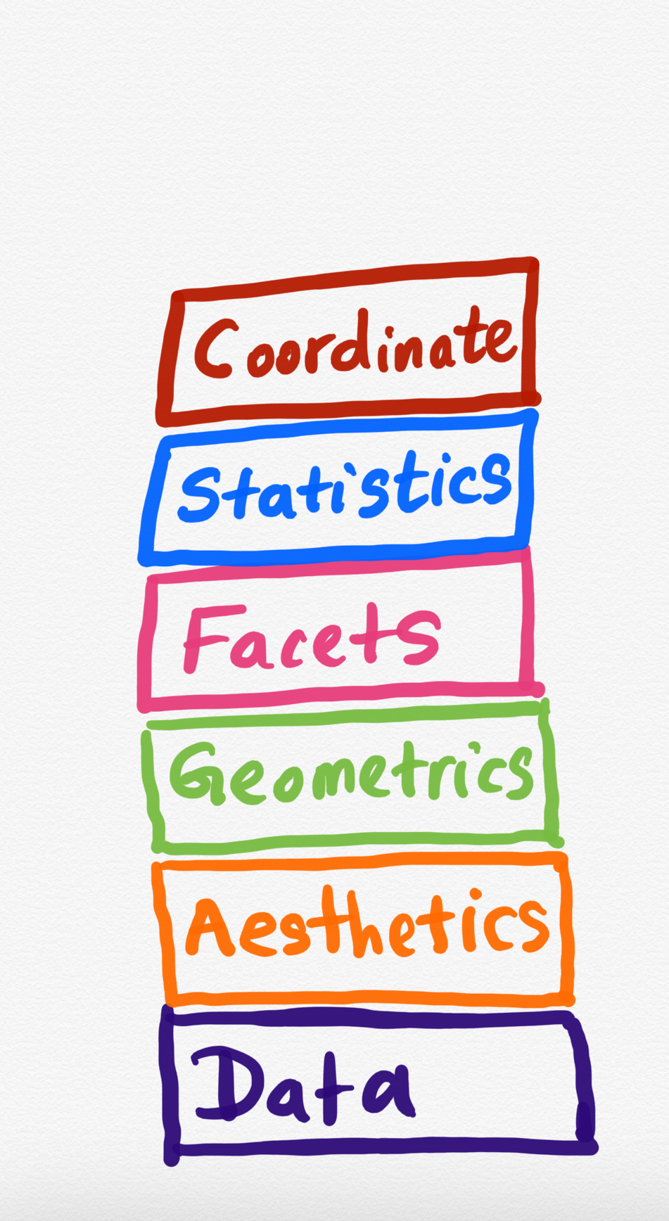
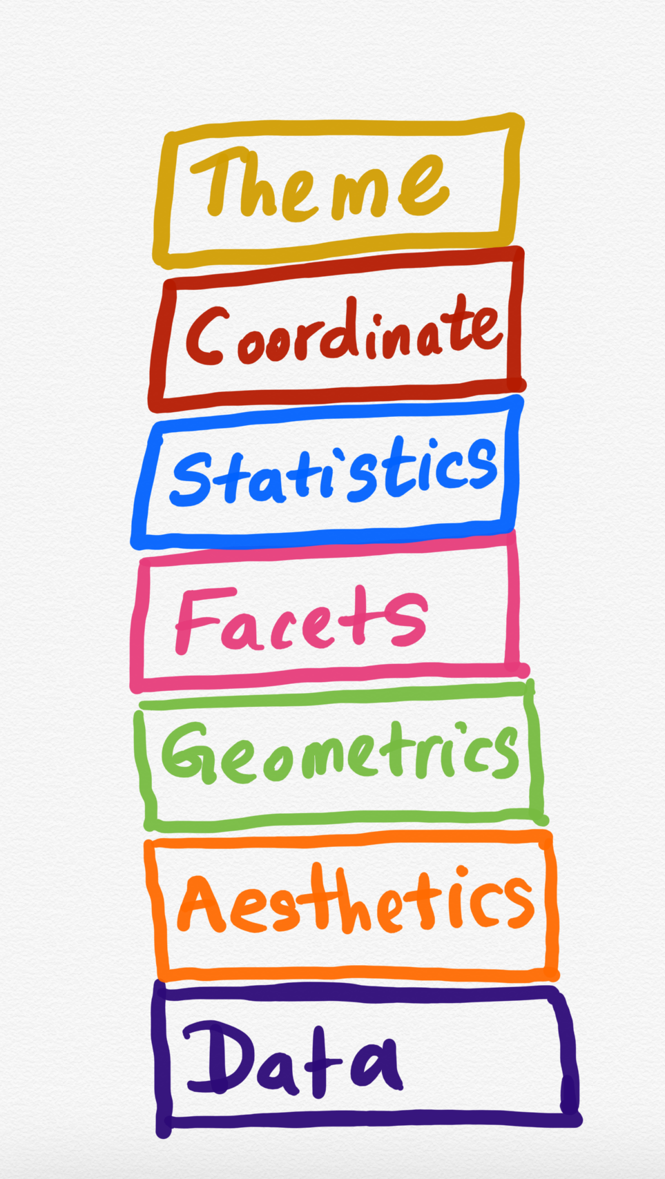
<ggplot: (-9223372036470736247)><ggplot: (-9223372036470265845)>Actual marks we put on a plot
<ggplot: (-9223372036469942633)><ggplot: (-9223372036469989246)><ggplot: (-9223372036469621511)><ggplot: (-9223372036469501724)>source: https://nbisweden.github.io/RaukR-2019/ggplot/presentation/ggplot_presentation.html#17
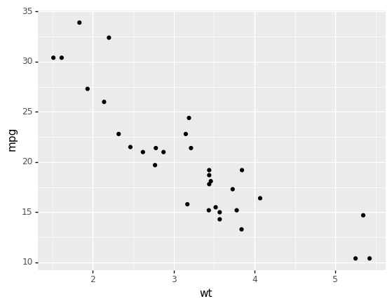
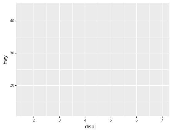
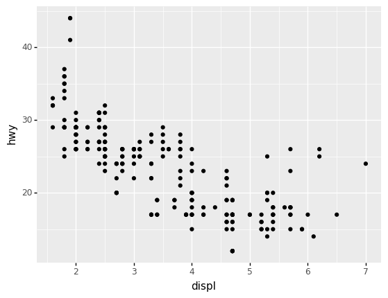
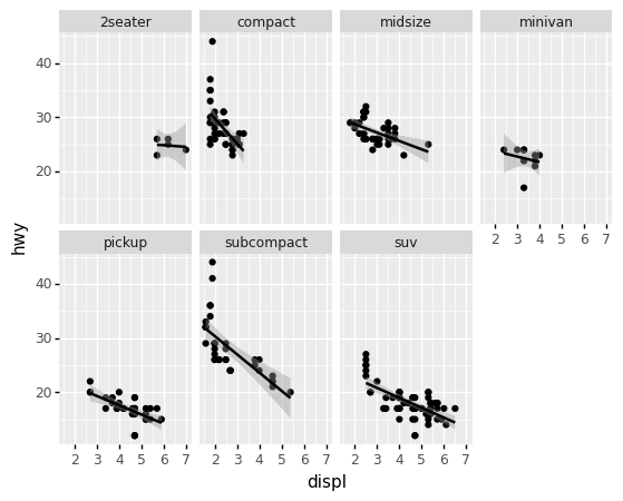
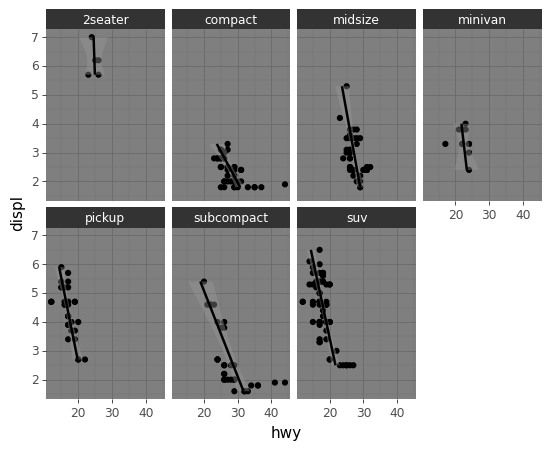
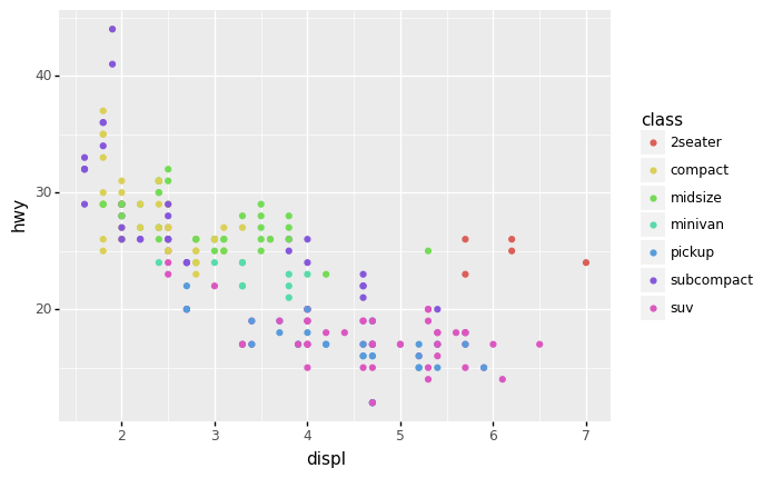
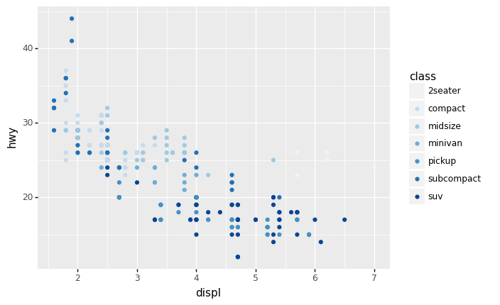
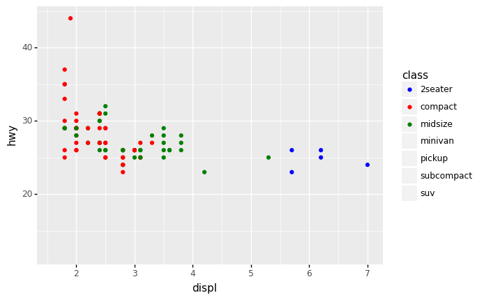
displ - a car’s engine size, in litres.
hwy - a car’s fuel efficiency on the highway, in miles per gallon (mpg)
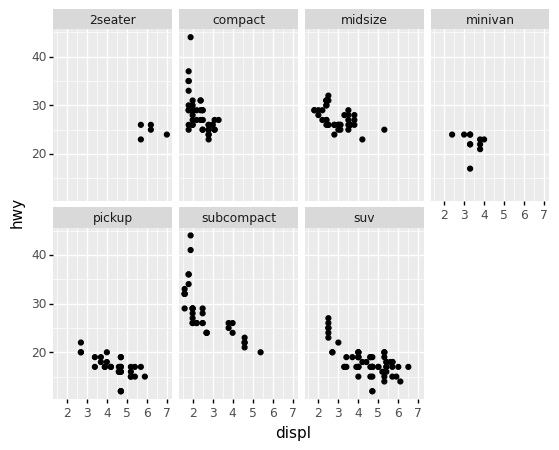
Subplots that each display one subset of the data.
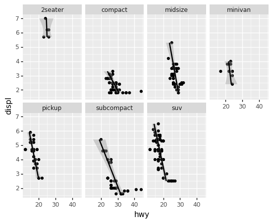
<ggplot: (-9223372036469377946)><ggplot: (383391510)>ggplot(mpg, aes(x='displ', y='hwy')) + geom_point() + facet_wrap("class", nrow=2)+ stat_smooth(method = "lm")<ggplot: (385913671)>ggplot(mpg, aes(x='displ', y='hwy')) + geom_point() + facet_wrap("class", nrow=2)+ stat_smooth(method = "lm") + coord_flip()<ggplot: (385251876)>ggplot(mpg, aes(x='displ', y='hwy')) + geom_point() + facet_wrap("class", nrow=2)+ stat_smooth(method = "lm") + coord_flip() + theme_dark()<ggplot: (383847323)><ggplot: (383894269)>ggplot(mpg, aes(x='displ', y='hwy', color='class')) + geom_point() + scale_color_manual(values=['blue', 'red', 'green'])<ggplot: (-9223372036468854114)>