Week 3-4: AR/ MA/ ARMA/ ARIMA

Recap: Stationarity

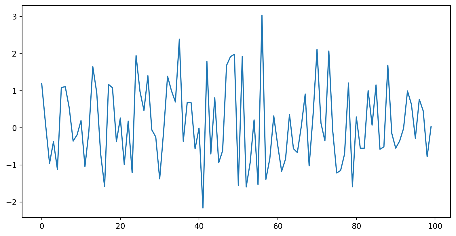
import numpy
import matplotlib.pyplot as plt

mean = 0
std = 1 
num_samples = 100
samples = numpy.random.normal(mean, std, size=num_samples)
plt.plot(samples)
plt.show()

ACF

White noise implies stationarity. Stationarity does not imply white noise.

Non-Stationary Time Series

1. Deterministic trend

\[Y_t = f(t) + \epsilon_t\]

where \(\epsilon_t \sim iid(0, \sigma^2)\), \(t = 1, 2, ...T\)

Mean of the process is time dependent, but the variance of the process is constant.

A trend is deterministic if it is a nonrandom function of time.

Non-Stationary Time Series (cont.)

2. Random walk

\[Y_t = Y_{t-1} + \epsilon_t\]

• Random walk has a stochastic trend.

• Model behind naive method.

A trend is said to be stochastic if it is a random function of time.

Non-Stationary Time Series (cont.)

3. Random walk with drift

\[Y_t = \alpha+ Y_{t-1} + \epsilon_t\]

• Random walk with drift has a stochastic trend and a deterministic trend.

• Model behind drift method.

Random walk

\[ \begin{aligned} Y_t &= Y_{t-1} + \epsilon_t \\ Y_1 &= Y_0 + \epsilon_1 \\ Y_2 &= Y_1 + \epsilon_2=Y_0 + \epsilon_1 + \epsilon_2\\ Y_3 &= Y_2 + \epsilon_3=Y_0 + \epsilon_1 + \epsilon_2 +\epsilon_3\\ . \\ Y_t &=Y_{t-1} + \epsilon_t=Y_0 + \epsilon_1 + \epsilon_2 + \epsilon_3 +...+ \epsilon_t = Y_0 + \sum_{i=1}^{t} \epsilon_t \end{aligned} \]

Mean: \(E(Y_t) = Y_0\).

Variance: \(Var(Y_t)=t \sigma^2\).

Random walk with drift

\[ \begin{aligned} Y_t &= Y_{t-1} + \epsilon_t \\ Y_1 &= \alpha+Y_0 + \epsilon_1 \\ Y_2 &= \alpha+ Y_1 + \epsilon_2=2 \alpha+Y_0 + \epsilon_1 + \epsilon_2\\ Y_3 &= \alpha+ Y_2 + \epsilon_3= 3 \alpha+ Y_0 + \epsilon_1 + \epsilon_2 +\epsilon_3\\ . \\ Y_t &= \alpha+Y_{t-1} + \epsilon_t= t \alpha+ Y_0 + \epsilon_1 + \epsilon_2 + \epsilon_3 +...+ \epsilon_t \\ Y_t &= t \alpha + Y_0 + \sum_{i=1}^{t} \epsilon_t \end{aligned} \]

Random walk with drift (cont.)

It has a deterministic trend \((Y_0 + t \alpha)\) and a stochastic trend \(\sum_{i=1}^{t} \epsilon_t\).

Mean: \(E(Y_t) = Y_0 + t\alpha\)

Variance: \(Var(Y_t) = t\sigma^2\).

There is a trend in both mean and variance.

Common trend removal (de-trending) procedures

1. Deterministic trend: Time-trend regression

   The trend can be removed by fitting a deterministic polynomial time trend. The residual series after removing the trend will give us the de-trended series.

2. Stochastic trend: Differencing

   The process is also known as a Difference-stationary process.

Notation: I(d)

Integrated to order \(d\): Series can be made stationary by differencing \(d\) times.

• Known as \(I(d)\) process.

Question: Show that random walk process is an \(I(1)\) process.

The random walk process is called a unit root process. (If one of the roots turns out to be one, then the process is called unit root process.)

Random walk

import numpy as np
rw = np.cumsum(samples)
plt.plot(rw)
plt.show()

Random walk - ACF

Difference series

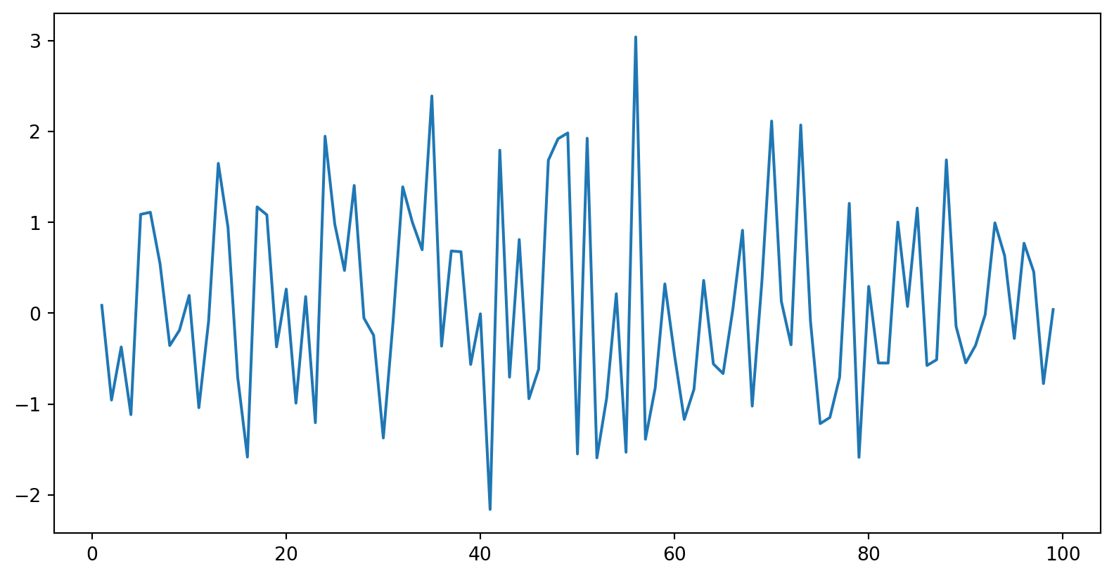
	Values	Lag 1	Lag 2
0	1.203587	NaN	NaN
1	1.290288	0.086700	NaN
2	0.334784	-0.955504	-1.042204
3	-0.036386	-0.371170	0.584334
4	-1.152387	-1.116001	-0.744831
...	...	...	...
95	10.696335	-0.277457	-0.910943
96	11.466986	0.770650	1.048107
97	11.923566	0.456580	-0.314070
98	11.149137	-0.774429	-1.231009
99	11.190200	0.041062	0.815491

100 rows × 3 columns

Plot Lag 1 series

ACF Lag 1 series

Example 2

import numpy as np, pandas as pd
from statsmodels.graphics.tsaplots import plot_acf, plot_pacf
import matplotlib.pyplot as plt
plt.rcParams.update({'figure.figsize':(9,7), 'figure.dpi':120})

# Import data
df = pd.read_csv('wwwusage.csv', names=['value'], header=0)

# Original Series
fig, axes = plt.subplots(2, 2, sharex=True)
axes[0, 0].plot(df.value); axes[0, 0].set_title('Original Series')
plot_acf(df.value, ax=axes[0, 1], lags=np.arange(len(df)))

# 1st Differencing
axes[1, 0].plot(df.value.diff()); axes[1, 0].set_title('1st Order Differencing')
plot_acf(df.value.diff().dropna(), ax=axes[1, 1], lags=np.arange(len(df) - 1))
plt.show()

2nd order differencing

plot_acf(df.value.diff().diff().dropna())
plt.show()

Variance stabilization

Eg:

• Square root: \(W_t = \sqrt{Y_t}\)

• Logarithm: \(W_t = log({Y_t})\)

  • This very useful.

  • Interpretable: Changes in a log value are relative (percent) changes on the original sclae.

Monthly Airline Passenger Numbers 1949-1960

airpassenger = pd.read_csv('AirPassengers.csv')
from datetime import datetime
import plotnine
from plotnine import *
airpassenger['Month']= pd.to_datetime(airpassenger['Month'])
ggplot(airpassenger, aes(x='Month', y='#Passengers'))+geom_line()

<ggplot: (331734342)>

Monthly Airline Passenger Numbers 1949-1960 - log

import numpy as np
airpassenger['naturallog'] = np.log(airpassenger['#Passengers']) 
ggplot(airpassenger, aes(x='Month', y='naturallog'))+geom_line()

<ggplot: (331805001)>

Box-Cox transformation

\[ w_t=\begin{cases} log(y_t), & \text{if $\lambda=0$} \newline (Y_t^\lambda - 1)/ \lambda, & \text{otherwise}. \end{cases} \]

Different values of \(\lambda\) gives you different transformations.

• \(\lambda=1\): No substantive transformation

• \(\lambda = \frac{1}{2}\): Square root plus linear transformation

• \(\lambda=0\): Natural logarithm

• \(\lambda = -1\): Inverse plus 1

Balance the seasonal fluctuations and random variation across the series.

Box-Cox transformation

# import modules
import numpy as np
from scipy import stats
 
y2,fitted_lambda = stats.boxcox(airpassenger['#Passengers'])

Box-Cox transformation: Exploring the output

fitted_lambda

0.14802265137037945

y2

array([ 6.82749005,  6.93282224,  7.16189151,  7.11461078,  6.98378687,
        7.20826542,  7.39959794,  7.39959794,  7.22352834,  6.94993188,
        6.67930112,  6.93282224,  6.88074148,  7.0663838 ,  7.29843847,
        7.20826542,  7.05009066,  7.41371485,  7.69297755,  7.69297755,
        7.53726005,  7.17744836,  6.86312389,  7.28363955,  7.35675408,
        7.42775127,  7.791663  ,  7.6033268 ,  7.71801394,  7.791663  ,
        8.03379957,  8.03379957,  7.86322651,  7.59025293,  7.3711186 ,
        7.64214252,  7.70552693,  7.81574285,  7.96693012,  7.82769741,
        7.85143867,  8.23478523,  8.35415797,  8.46833738,  8.14152446,
        7.94424651,  7.71801394,  7.97819691,  8.00058286,  8.00058286,
        8.41186604,  8.40233549,  8.34441554,  8.47763304,  8.66568618,
        8.73398286,  8.42136224,  8.16254066,  7.81574285,  8.05570781,
        8.08822445,  7.90983871,  8.40233549,  8.32482145,  8.39277032,
        8.66568618,  8.97573698,  8.90544371,  8.62209995,  8.34441554,
        8.0774311 ,  8.34441554,  8.46833738,  8.38317027,  8.69150146,
        8.70857469,  8.71707079,  9.07418456,  9.41661628,  9.30252389,
        9.05177744,  8.75078932,  8.42136224,  8.78409104,  8.83328615,
        8.77580407,  9.08902184,  9.0592668 ,  9.0964106 ,  9.48162515,
        9.72179099,  9.67415098,  9.35679401,  9.00640692,  8.72554012,
        9.00640692,  9.07418456,  8.96801544,  9.36350433,  9.30936559,
        9.35679401,  9.77445522, 10.01359054, 10.02424732,  9.66813973,
        9.30252389,  8.9987716 ,  9.22613489,  9.25415593,  9.0964106 ,
        9.40343224,  9.30936559,  9.41003199,  9.84886109, 10.14918625,
       10.21968352,  9.66813973,  9.38353935,  9.03673716,  9.23316669,
        9.390186  ,  9.26806127,  9.68014959,  9.61958794,  9.76283534,
       10.05072014, 10.426264  , 10.4768849 , 10.00289463,  9.68613564,
        9.40343224,  9.67415098,  9.74531682,  9.58881702,  9.75700771,
        9.99215929, 10.05072014, 10.36531089, 10.75145254, 10.68404894,
       10.23457308,  9.99215929,  9.58262264,  9.83186035])

ARMA(p, q) model

\[Y_t=c+\phi_1Y_{t-1}+...+\phi_p Y_{t-p}+ \theta_1\epsilon_{t-1}+...+\theta_q\epsilon_{t-q}+\epsilon_t\]

• These are stationary models.

• They are only suitable for stationary series.

ARIMA(p, d, q) model

Differencing –> ARMA

Step 1: Differencing

\[Y'_t = (1-B)^dY_t\]

Step 2: ARMA

\[Y'_t=c+\phi_1Y'_{t-1}+...+\phi_p Y'_{t-p}+ \theta_1\epsilon_{t-1}+...+\theta_q\epsilon_{t-q}+\epsilon_t\]

Step 1: Plot data

1. Detect unusual observations in the data

2. Detect non-stationarity by visual inspections of plots

Stationary series:

• has a constant mean value and fluctuates around the mean.

• constant variance.

• no pattern predictable in the long-term.

(<Figure size 1920x480 with 1 Axes>,
 <AxesSubplot: ylabel='Number of airline passengers'>)

Step 2: Split time series into training and test

Specify the forecast horizon

import numpy as np
import pandas as pd
from sktime.forecasting.base import ForecastingHorizon
fh = ForecastingHorizon(
    pd.PeriodIndex(pd.date_range("1960-01", periods=12, freq="M")), is_relative=False
)
fh

ForecastingHorizon(['1960-01', '1960-02', '1960-03', '1960-04', '1960-05', '1960-06',
             '1960-07', '1960-08', '1960-09', '1960-10', '1960-11', '1960-12'],
            dtype='period[M]', is_relative=False)

Plot training and test series

(<Figure size 1920x480 with 1 Axes>,
 <AxesSubplot: ylabel='Number of airline passengers'>)

1. Need transformations?

2. Need differencing?

Step 3: Apply transformations

import numpy as np
y_train.naturallog = np.log(y_train) 
plot_series(y_train.naturallog)

(<Figure size 1920x480 with 1 Axes>,
 <AxesSubplot: ylabel='Number of airline passengers'>)

Step 4: Take difference series

Identifying non-stationarity by looking at plots

• Time series plot

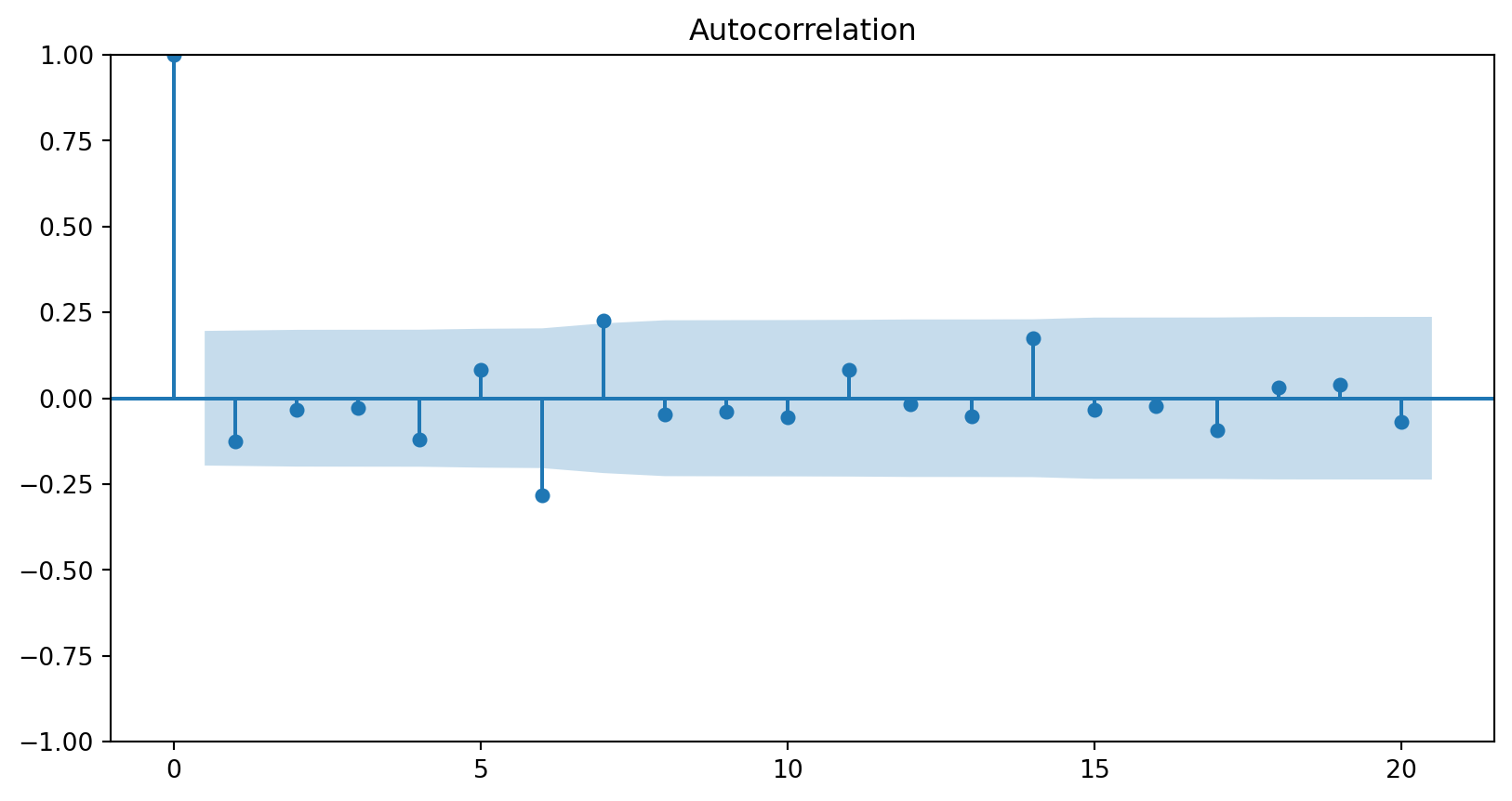
• The ACF of stationary data drops to zero relatively quickly.

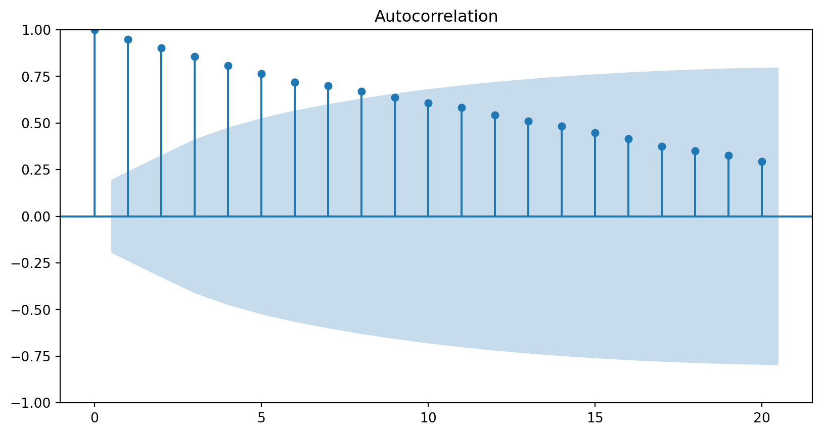
• The ACF of non-stationary data decreases slowly.

• For non-stationary data, the value of \(r_1\) is often large and positive.

Non-seasonal differencing and seasonal differencing

Non seasonal first-order differencing: \(Y'_t=Y_t - Y_{t-1}\)

Non seasonal second-order differencing: \(Y''_t=Y'_t - Y'_{t-1}\)

Seasonal differencing: \(Y_t - Y_{t-m}\)

• For monthly, \(m=12\), for quarterly, \(m=4\).

• Seasonally differenced series will have \(T-m\) observations.

There are times differencing once is not enough. However, in practice,it is almost never necessary to go beyond second-order differencing.

ACF of log-transformation series

plot_acf(y_train.naturallog, lags=50)

Take seasonal difference series

y_train.naturallog.diff12 = y_train.naturallog.diff(12)
y_train.naturallog.diff12

1949-01         NaN
1949-02         NaN
1949-03         NaN
1949-04         NaN
1949-05         NaN
             ...   
1959-08    0.101591
1959-09    0.136312
1959-10    0.125491
1959-11    0.155072
1959-12    0.183804
Freq: M, Name: Number of airline passengers, Length: 132, dtype: float64

Take seasonal difference series (cont.)

y_train.naturallog.diff12.head(20)

1949-01         NaN
1949-02         NaN
1949-03         NaN
1949-04         NaN
1949-05         NaN
1949-06         NaN
1949-07         NaN
1949-08         NaN
1949-09         NaN
1949-10         NaN
1949-11         NaN
1949-12         NaN
1950-01    0.026433
1950-02    0.065597
1950-03    0.065958
1950-04    0.045462
1950-05    0.032523
1950-06    0.098672
1950-07    0.138586
1950-08    0.138586
Freq: M, Name: Number of airline passengers, dtype: float64

ACF - diff(log(data), 12)

plot_acf(y_train.naturallog.diff12.dropna(), lags=50)
plt.show()

ACF - First differencing on diff(log(data), 12)

y_train.naturallog.diff12.diff = y_train.naturallog.diff12.diff()
plot_acf(y_train.naturallog.diff12.diff.dropna(), lags=50)
plt.show()

PACF - First differencing on diff(log(data), 12)

plot_pacf(y_train.naturallog.diff12.diff.dropna(), lags=50)
plt.show()

Testing for nonstationarity for the presence of unit roots

• Dickey and Fuller (DF) test

• Augmented DF test

• Phillips and Perron (PP) nonparametric test

• Kwiatkowski-Phillips-Schmidt-Shin (KPSS) test

KPSS test

H0: Series is level or trend stationary.

H1: Series is not stationary.

KPSS test

from statsmodels.tsa.stattools import kpss
def kpss_test(series, **kw):    
    statistic, p_value, n_lags, critical_values = kpss(series, **kw)
    # Format Output
    print(f'KPSS Statistic: {statistic}')
    print(f'p-value: {p_value}')
    print(f'num lags: {n_lags}')
    print('Critial Values:')
    for key, value in critical_values.items():
        print(f'   {key} : {value}')
    print(f'Result: The series is {"not " if p_value < 0.05 else ""}stationary')

kpss_test(y_train.naturallog)

KPSS Statistic: 1.9204939010623039
p-value: 0.01
num lags: 6
Critial Values:
   10% : 0.347
   5% : 0.463
   2.5% : 0.574
   1% : 0.739
Result: The series is not stationary

KPSS test

kpss_test(y_train.naturallog.diff12.dropna())

KPSS Statistic: 0.29885781439314946
p-value: 0.1
num lags: 5
Critial Values:
   10% : 0.347
   5% : 0.463
   2.5% : 0.574
   1% : 0.739
Result: The series is stationary

kpss_test(y_train.naturallog.diff12.diff.dropna())

KPSS Statistic: 0.0509726778456186
p-value: 0.1
num lags: 2
Critial Values:
   10% : 0.347
   5% : 0.463
   2.5% : 0.574
   1% : 0.739
Result: The series is stationary

KPSS test

• KPSS test may not necessarily reject the null hypothesis (that the series is level or trend stationary) even if a series is steadily increasing or decreasing.

• The word ‘deterministic’ implies the slope of the trend in the series does not change permanently. That is, even if the series goes through a shock, it tends to regain its original path.

source: https://www.machinelearningplus.com/time-series/kpss-test-for-stationarity/

KPSS test

• By default, it tests for stationarity around a ‘mean’ only.

• To turn ON the stationarity testing around a trend, you need to explicitly pass the regression=‘ct’ parameter to the kpss

kpss_test(y_train.naturallog.diff12.dropna(), regression='ct')

KPSS Statistic: 0.0760056301424143
p-value: 0.1
num lags: 5
Critial Values:
   10% : 0.119
   5% : 0.146
   2.5% : 0.176
   1% : 0.216
Result: The series is stationary

kpss_test(y_train.naturallog.diff12.diff.dropna())

KPSS Statistic: 0.0509726778456186
p-value: 0.1
num lags: 2
Critial Values:
   10% : 0.347
   5% : 0.463
   2.5% : 0.574
   1% : 0.739
Result: The series is stationary

ADF test

from statsmodels.tsa.stattools import adfuller

def adf_test(series):
    result = adfuller(series, autolag='AIC')
    print(f'ADF Statistic: {result[0]}')
    print(f'p-value: {result[1]}')
    for key, value in result[4].items():
        print('Critial Values:')
        print(f'   {key}, {value}')

series = df.loc[:, 'value'].values

H0: Series is not stationary

H1: Series is stationary

ADF test

adf_test(y_train.naturallog)

ADF Statistic: -1.3176112021439967
p-value: 0.6210771494355872
Critial Values:
   1%, -3.4870216863700767
Critial Values:
   5%, -2.8863625166643136
Critial Values:
   10%, -2.580009026141913

adf_test(y_train.naturallog.diff12.dropna())

ADF Statistic: -2.5844902417566793
p-value: 0.09624537566648711
Critial Values:
   1%, -3.492995948509562
Critial Values:
   5%, -2.888954648057252
Critial Values:
   10%, -2.58139291903223

adf_test(y_train.naturallog.diff12.diff.dropna())

ADF Statistic: -4.08727195454389
p-value: 0.0010165214009067135
Critial Values:
   1%, -3.4936021509366793
Critial Values:
   5%, -2.8892174239808703
Critial Values:
   10%, -2.58153320754717

KPSS vs ADF test

If a series is stationary according to the KPSS test by setting regression=‘ct’ and is not stationary according to the ADF test, it means the series is stationary around a deterministic trend.

Further reading:

Kwiatkowski, D.; Phillips, P. C. B.; Schmidt, P.; Shin, Y. (1992). Testing the null hypothesis of stationarity against the alternative of a unit root. Journal of Econometrics, 54 (1-3): 159-178.

Step 5: Examine the ACF/PACF to identify a suitable model

AR(p)

• ACF dies out in an exponential or damped sine-wave manner.

• there is a significant spike at lag \(p\) in PACF, but none beyond \(p\).

MA(q)

• ACF has all zero spikes beyond the \(q^{th}\) spike.

• PACF dies out in an exponential or damped sine-wave manner.

Seasonal components

• The seasonal part of an AR or MA model will be seen in the seasonal lags of the PACF and ACF.

ARIMA(0,0,0)(0,0,1)12 will show

• a spike at lag 12 in the ACF but no other significant spikes.

• The PACF will show exponential decay in the seasonal lags 12, 24, 36, . . . .

ARIMA(0,0,0)(1,0,0)12 will show

• exponential decay in the seasonal lags of the ACF.

• a single significant spike at lag 12 in the PACF.

Step 5: Examine the ACF/PACF to identify a suitable model (cont.)

• \(d=1\) and \(D=1\) (from step 4)

• Significant spike at lag 1 in ACF suggests non-seasonal MA(1) component.

• Significant spike at lag 12 in ACF suggests seasonal MA(1) component.

• Initial candidate model: \(ARIMA(0,1,1)(0,1,1)_{12}\).

• By analogous logic applied to the PACF, we could also have started with \(ARIMA(1,1,0)(1,1,0)_{12}\).

Models

Initial model:

\(ARIMA(0,1,1)(0,1,1)_{12}\)

\(ARIMA(1,1,0)(1,1,0)_{12}\)

Try some variations of the initial model:

\(ARIMA(0,1,1)(1,1,1)_{12}\)

\(ARIMA(1,1,1)(1,1,0)_{12}\)

\(ARIMA(1,1,1)(1,1,1)_{12}\)

Try some variations

Both the ACF and PACF show significant spikes at lag 3, and almost significant spikes at lag 3, indicating that some additional non-seasonal terms need to be included in the model.

\(ARIMA(3,1,1)(1,1,1)_{12}\)

\(ARIMA(1,1,3)(1,1,1)_{12}\)

\(ARIMA(3,1,3)(1,1,1)_{12}\)

Fitting ARIMA models

from sktime.forecasting.arima import ARIMA
forecaster1 = ARIMA(  
    order=(1, 1, 0),
    seasonal_order=(1, 1, 0, 12),
    suppress_warnings=True)
forecaster1.fit(y_train.naturallog)    

ARIMA(order=(1, 1, 0), seasonal_order=(1, 1, 0, 12), suppress_warnings=True)

In a Jupyter environment, please rerun this cell to show the HTML representation or trust the notebook.
On GitHub, the HTML representation is unable to render, please try loading this page with nbviewer.org.

Step 6: Check residual series

fhtrain = ForecastingHorizon(
    pd.PeriodIndex(pd.period_range(start='1949-01', end='1959-12', freq='M')), is_relative=False
)
fhtrain

ForecastingHorizon(['1949-01', '1949-02', '1949-03', '1949-04', '1949-05', '1949-06',
             '1949-07', '1949-08', '1949-09', '1949-10',
             ...
             '1959-03', '1959-04', '1959-05', '1959-06', '1959-07', '1959-08',
             '1959-09', '1959-10', '1959-11', '1959-12'],
            dtype='period[M]', length=132, is_relative=False)

Obtain predictions for the training period

y_pred_train = forecaster1.predict(fhtrain)
y_pred_train

1949-01         NaN
1949-02    4.718760
1949-03    4.770946
1949-04    4.883063
1949-05    4.860073
             ...   
1959-08    6.310106
1959-09    6.138659
1959-10    6.004945
1959-11    5.869054
1959-12    5.974289
Freq: M, Length: 132, dtype: float64

Obtain residual series

residual = y_train.naturallog - y_pred_train
residual

1949-01         NaN
1949-02    0.051925
1949-03    0.111856
1949-04   -0.023251
1949-05   -0.064283
             ...   
1959-08    0.016043
1959-09   -0.000931
1959-10    0.003868
1959-11    0.022590
1959-12    0.029598
Freq: M, Length: 132, dtype: float64

Plot residuals

plot_series(residual)

(<Figure size 1920x480 with 1 Axes>, <AxesSubplot: >)

Plot residuals (cont.)

plot_acf(residual.dropna(), lags=50)

Plot residuals (cont.)

import matplotlib.pyplot as plt
import numpy as np
plt.hist(residual)
plt.show()

Your turn: remove the outlier and draw the histogram

Ljung-Box Test

H0: Residuals are not serially correlated.

H1: Residuals are serially correlated.

	lb_stat	lb_pvalue
20	3.984776	0.999955

Step 7: Generate forecasts

y_pred_1 = forecaster1.predict(fh)
y_pred_1

1960-01    6.037478
1960-02    5.982107
1960-03    6.133707
1960-04    6.102795
1960-05    6.154218
1960-06    6.301004
1960-07    6.437653
1960-08    6.461717
1960-09    6.257650
1960-10    6.134112
1960-11    6.003672
1960-12    6.103036
Freq: M, dtype: float64

Back transformation

y_pred_1.exp = np.exp(y_pred_1)
y_pred_1.exp

1960-01    418.835520
1960-02    396.274338
1960-03    461.142677
1960-04    447.105543
1960-05    470.698677
1960-06    545.118980
1960-07    624.938414
1960-08    640.159214
1960-09    521.990600
1960-10    461.329316
1960-11    404.912933
1960-12    447.213408
Freq: M, dtype: float64

Plot training, test, and forecasts

plot_series(y_train, y_test, y_pred_1.exp, labels=["y_train", "y_test", "y_forecast"])

(<Figure size 1920x480 with 1 Axes>,
 <AxesSubplot: ylabel='Number of airline passengers'>)

Evaluation

from sktime.performance_metrics.forecasting import \
    mean_absolute_percentage_error
mean_absolute_percentage_error(y_test, y_pred_1.exp, symmetric=False)

0.027756916452706674

Your Turn

Fit other variants of ARIMA models and identify the best ARIMA model for the series.

Modelling steps

1. Plot the data.

2. If necessary, transform the data (using a Box-Cox transformation) to stabilise the variance.

3. If the data are non-stationary, take first differences of the data until the data are stationary.

4. Examine the ACF/PACF to identify a suitable model.

5. Try your chosen model(s), and use the AICc to search for a better model.

Modelling steps (cont.)

6. Check the residuals from your chosen model by plotting the ACF of the residuals, and doing a portmanteau test of the residuals. If they do not look like white noise, try a modified model.

7. Once the residuals look like white noise, calculate forecasts.

Source: Forecasting: Principles and Practice, Rob J Hyndman and George Athanasopoulos