from sktime import *
from sktime.datasets import load_airline
from sktime.utils.plotting import plot_series
y = load_airline()
plot_series(y)
(<Figure size 1536x384 with 1 Axes>,
<AxesSubplot: ylabel='Number of airline passengers'>)
Plot the data.
If necessary, transform the data (using a Box-Cox transformation) to stabilise the variance.
3. If the data are non-stationary, take first differences of the data until the data are stationary.
4. Examine the ACF/PACF to identify a suitable model.
5. Try your chosen model(s), and use the AICc to search for a better model.
Check the residuals from your chosen model by plotting the ACF of the residuals, and doing a portmanteau test of the residuals. If they do not look like white noise, try a modified model.
Once the residuals look like white noise, calculate forecasts.
Plot the data.
If necessary, transform the data (using a Box-Cox transformation) to stabilise the variance.
Use AutoARIMA to select a model.
Check the residuals from your chosen model by plotting the ACF of the residuals, and doing a portmanteau test of the residuals. If they do not look like white noise, try a modified model.
Once the residuals look like white noise, calculate forecasts.
Take other important visualizations
import numpy as np
import pandas as pd
from sktime.forecasting.base import ForecastingHorizon
fh = ForecastingHorizon(
pd.PeriodIndex(pd.date_range("1960-01", periods=12, freq="M")), is_relative=False
)
fh
ForecastingHorizon(['1960-01', '1960-02', '1960-03', '1960-04', '1960-05', '1960-06',
'1960-07', '1960-08', '1960-09', '1960-10', '1960-11', '1960-12'],
dtype='period[M]', is_relative=False)
from sktime.forecasting.statsforecast import StatsForecastAutoARIMA
import numpy as np
forecaster = StatsForecastAutoARIMA(
sp=12, max_p=2, max_q=2
)
y_train.naturallog = np.log(y_train)
forecaster.fit(y_train.naturallog)
StatsForecastAutoARIMA(max_p=2, max_q=2, sp=12)In a Jupyter environment, please rerun this cell to show the HTML representation or trust the notebook.
StatsForecastAutoARIMA(max_p=2, max_q=2, sp=12)
sp: Number of observations per unit of time.
Help: https://www.sktime.org/en/stable/api_reference/auto_generated/sktime.forecasting.statsforecast.StatsForecastAutoARIMA.html
Preferm residual analysis
Coverage | ||
---|---|---|
0.9 | ||
lower | upper | |
1960-01 | 5.978520 | 6.099244 |
1960-02 | 5.916820 | 6.062361 |
1960-03 | 6.062679 | 6.229384 |
1960-04 | 6.026940 | 6.212408 |
1960-05 | 6.058205 | 6.260705 |
1960-06 | 6.195598 | 6.413804 |
1960-07 | 6.316247 | 6.549103 |
1960-08 | 6.321487 | 6.568124 |
1960-09 | 6.136959 | 6.396648 |
1960-10 | 6.000121 | 6.272235 |
1960-11 | 5.865717 | 6.149713 |
1960-12 | 5.966786 | 6.262187 |
y_test.naturallog = np.log(y_test)
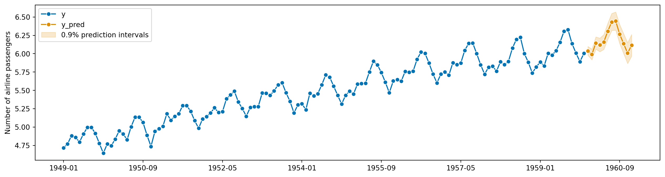
from sktime.utils import plotting
# also requires predictions
y_pred = forecaster.predict()
fig, ax = plotting.plot_series(y_train.naturallog, y_pred, labels=["y", "y_pred"])
ax.fill_between(
ax.get_lines()[-1].get_xdata(),
y_pred_ints["Coverage"][coverage]["lower"],
y_pred_ints["Coverage"][coverage]["upper"],
alpha=0.2,
color=ax.get_lines()[-1].get_c(),
label=f"{coverage}% prediction intervals",
)
ax.legend();
Step 1: Select the number of differences d and D via unit root tests and strength of seasonality measure.
Step 2: Try four possible models to start with:
ARIMA(2,d,2) if m=1 and ARIMA(2,d,2)(1,D,1)m if m>1.
ARIMA(0,d,0) if m=1 and ARIMA(0,d,0)(0,D,0)m if m>1.
ARIMA(1,d,0) if m=1 and ARIMA(1,d,0)(1,D,0)m if m>1.
ARIMA(0,d,1) if m=1 and ARIMA(0,d,1)(0,D,1)m if m>1.
Step 3: Select the model with the smallest AICc from step 2. This becomes the current model.
Step 4: Consider up to 13 variations on the current model:
Vary one of p,q,P and Q from the current model by ±1.
p,q both vary from the current model by ±1.
P,Q both vary from the current model by ±1.
Include or exclude the constant term from the current model. Repeat step 4 until no lower AICc can be found.