Time Series Clustering
Is the following series dissimilar or similar?
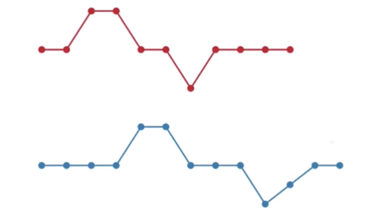
What is time series clustering?
Group similar time series
What we meant by similar?
similar profiles
similar features
same best forecasting models
similar data generating process
Before clustering think what is the purpose of grouping?
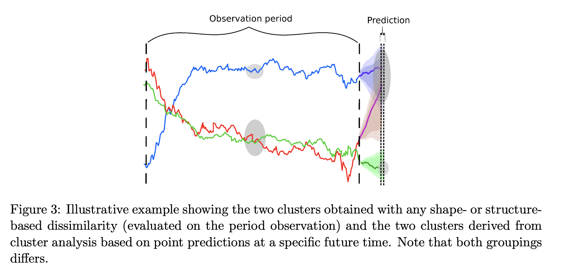 Source: Montero, P., & Vilar, J. A. (2015). TSclust: An R package for time series clustering. Journal of Statistical Software, 62, 1-43.
Time Series Clustering
Model-free approaches
Model-based approaches
Complexity-based approaches
Prediction-based approaches
Model-free approaches
\[\textbf{X}_T = (X_1, X_2, ..., X_T)^T\]
\[\textbf{Y}_T = (Y_1, Y_2, ..., Y_T)^T\]
Minkowski distance
\[d_{Lq}(\textbf{X}_T, \textbf{Y}_T) = [\sum_{t=1}^T(X_t, Y_t)^q]^{(\frac{1}{q})}\]
When \(q=1\) - Manhattan distance
When \(q=2\) - Euclidean distance
Observations are treated as independent. (\(d_{Lq}\) is invariant to permutation over time)
Very sensitive to time scaling
Frechet distance
Source: https://pure.tue.nl/ws/portalfiles/portal/93882810/Thesis_Tom_van_Diggelen.pdf
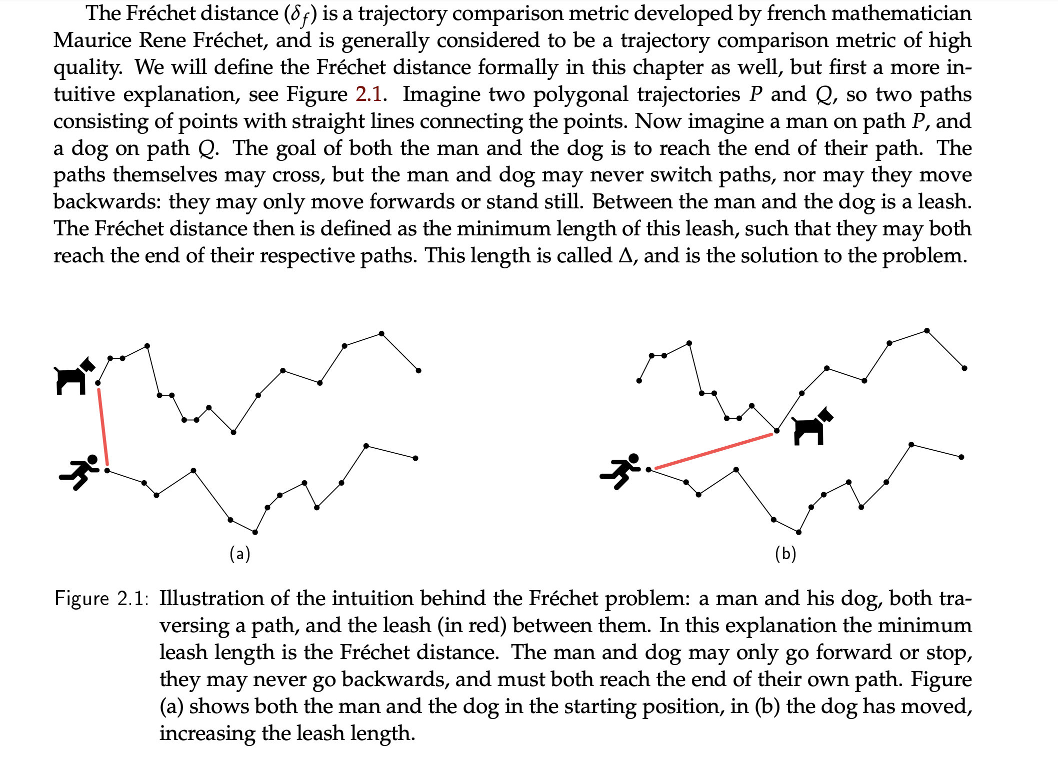
 Source: https://pure.tue.nl/ws/portalfiles/portal/93882810/Thesis_Tom_van_Diggelen.pdf
Frechet distance
The standard Fréchet distance is the minimum leash length required for the person to walk the dog without backtracking.
Account the ordering of the observations
Can be computed on series of different lengths
Dynamic time warping distance (DTW)
https://www.youtube.com/watch?v=ERKDHZyZDwA

Correlation-based distance
Pearson’s correlation between \(\textbf{X_T}\) and \(\textbf{Y_T}\): \(Cor(\textbf{X}_T, \textbf{Y}_T)\)
\[d_{cor1}= \sqrt{2(1-Cor(\textbf{X}_T, \textbf{Y}_T))}\]
\[d_{cor2}= \left (\left (\frac{1-Cor(\textbf{X}_T, \textbf{Y}_T)}{1+Cor(\textbf{X}_T, \textbf{Y}_T)} \right )^{\beta} \right )^{\frac{1}{2}}\]
where \(\beta \geq 0\).
Autocorrelation-based distance
Distance is based on estimated autocorrelation function.
Case 1: Uniform weight
\[d(\textbf{X}_T, \textbf{Y}_T) = \sqrt{\sum_{i=1}^L(\hat{\rho}_{i, X}-\hat{\rho}_{i, Y})^2}\]
Case 2: Geometric weights decaying with autocorrelation lag
\[d(\textbf{X}_T, \textbf{Y}_T) = \sqrt{\sum_{i=1}^Lw(1-w)^i(\hat{\rho}_{i, X}-\hat{\rho}_{i, Y})^2}\]
Periodogram-based distance
A periodogram is used to identify the dominant periods (or frequencies) of a time series.
Euclidean distance between the periodogram ordinates (Gives more weight to the shape of the curve)
Euclidean distance between the normalized periodogram ordinates (Consider the scale)
Reading: https://online.stat.psu.edu/stat510/lesson/6/6.1
Other model-free measures
Dissimilarity measures based on nonparametric spectral estimators
Dissimilarity measure based on wavelet transformation
Dissimilarity measure based on the symbolicrepresentation SAX
Model-based approaches
Piccolo distance
Invertible ARIMA processes
Euclidean distance between the \(AR(\infty)\)
In-class explanations.
Invertible condition
Backshift notation:
\[BX_t=X_{t-1}\] ARMA(p, q)
\[x_t= c+ \phi_1x_{t-1}+\phi_2x_{t-2}+...+\phi_px_{t-p} + \theta_1\epsilon_{t-1}+\theta_2\epsilon _{t-2}+...+\theta_q \epsilon_{t-q}+\epsilon_t,\]
\[x_t= c+ \phi_1Bx_{t}+\phi_2B^2x_{t}+...+\phi_pB^px_{t} + \theta_1B\epsilon_{t}+\theta_2B^2\epsilon _{t}+...+\theta_q B^q\epsilon_{t}+\epsilon_t,\] \[x_t - \phi_1Bx_{t}-\phi_2B^2x_{t}-...-\phi_pB^px_{t} = c + \theta_1B\epsilon_{t}+\theta_2B^2\epsilon _{t}+...+\theta_q B^q\epsilon_{t}+\epsilon_t,\]
\[\Phi(B)x_t = c+\Theta(B)\epsilon_t\]
\[\Phi(B)x_t = c+\Theta(B)\epsilon_t\]
\[\Phi(B) = 1-\phi_1B-\phi_2B^2-...-\phi_pB^p\]
\[\Theta(B)= 1+\theta_1B+\theta_2B^2 _{t}+...+\theta_q B^q\]
This process is called invertible if the modulus of all the roots of \(\Theta(B)=0\) are greater than one.
Demo
https://github.com/thiyangt/AR-infinite-coefficients/blob/master/ARinfinite-code.md
Maharaj distance
For the class of invertible and stationary ARMA processes
Based on hypotheses testing to determine whether or not two time series have significantly different generating processes
Two dissimilarity measures: one is based on test statistics, other one is based on the associated p-value
Prediction-based approaches
Two time series are similar if their forecasts at s specific future time are close.
Feature-based time series clustering
Link to slides: https://thiyangt.github.io/whyR2021keynote/#1
tsfeatures package in Python: https://pypi.org/project/tsfeatures/
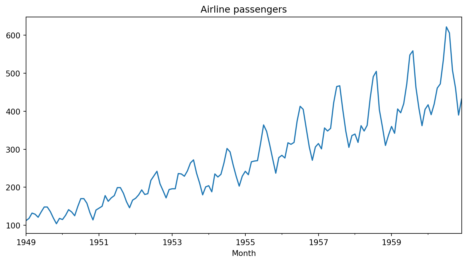
Data
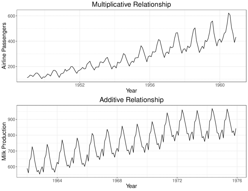
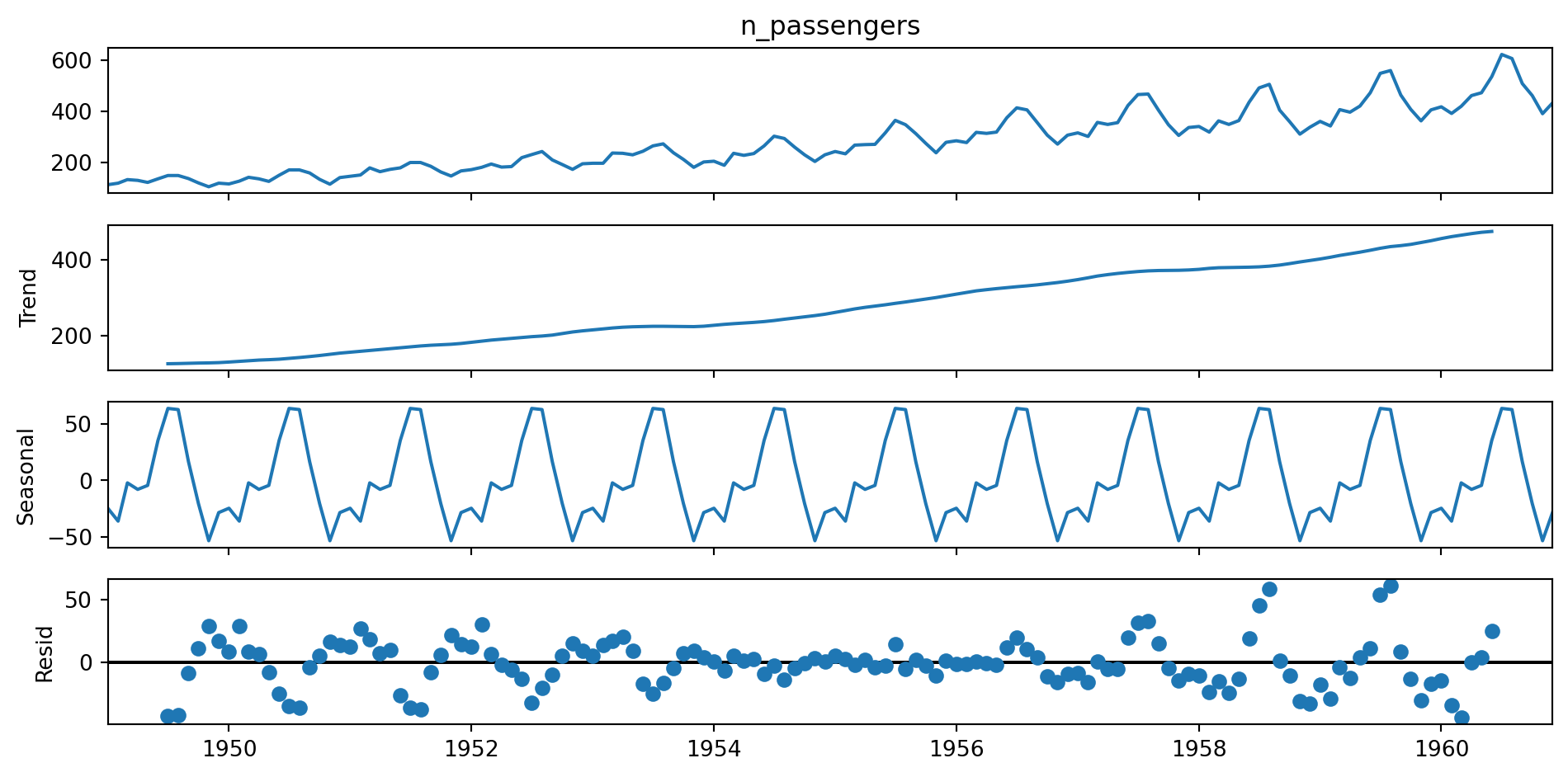
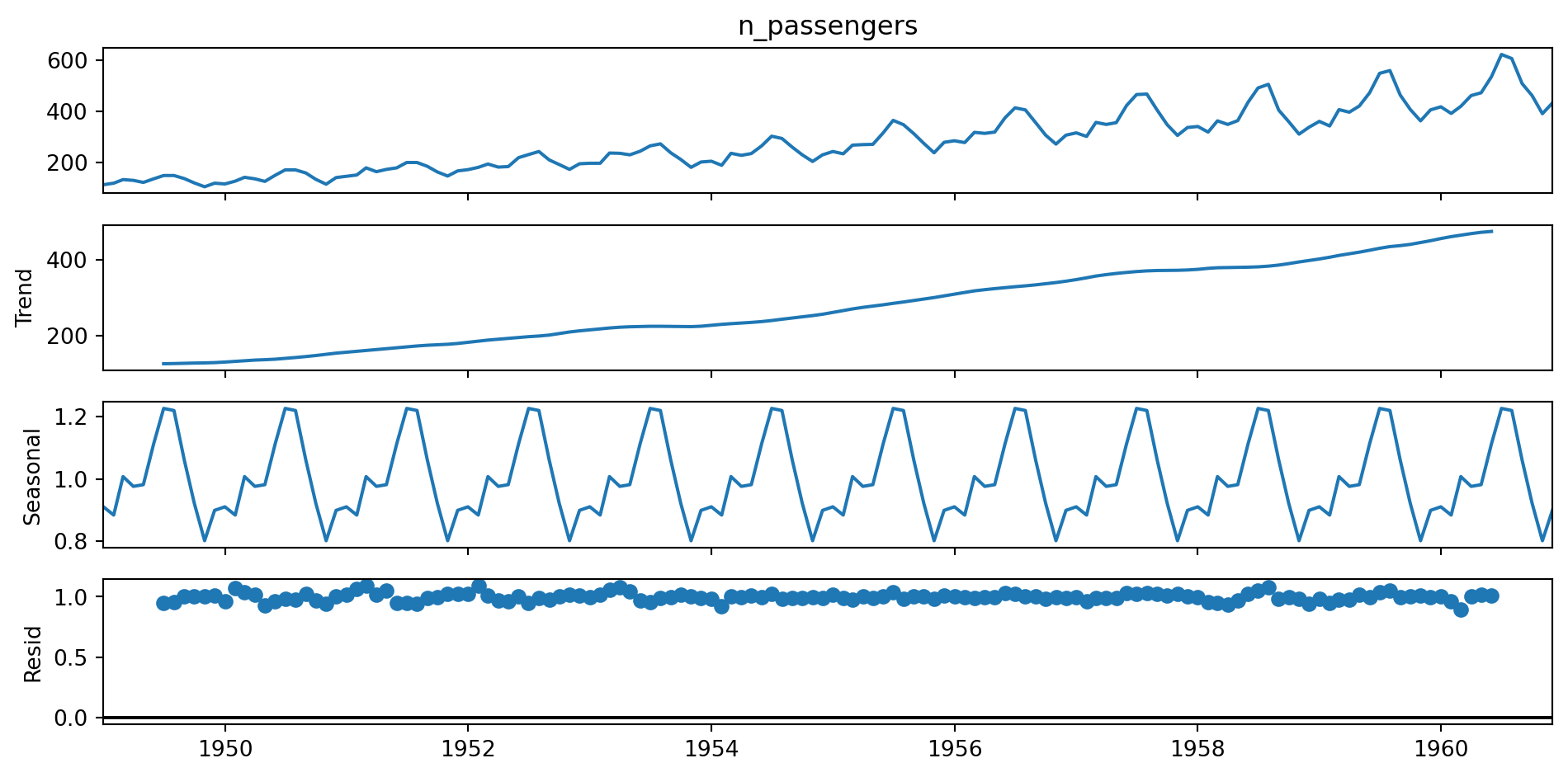
Additive and multiplicative seasonality – can you identify them correctly? https://kourentzes.com/forecasting/2014/11/09/additive-and-multiplicative-seasonality/
Time series features
Talagala, T. S., Hyndman, R. J., & Athanasopoulos, G. (2018). Meta-learning how to forecast time series. Monash Econometrics and Business Statistics Working Papers, 6(18), 16.
https://www.monash.edu/business/ebs/research/publications/ebs/wp06-2018.pdf
Complexity-based approaches
Compression-based dissimilarity measures
Permutation distribution clustering
Complexity-invariant dissimilarity measure
